How To Show Your Minority Class Much-Needed TLC
A comprehensive hands-on tutorial on class imbalance with coding examples in Python

In the post-Corona era with the worst definitely behind us here in NYC and the States, we should all first of all take some time to give ourselves some long overdue TLC, but once that is all said and done, let’s talk about how to give your minority class some proper TLC in your next classification project.
Throughout much of the latter half of my program at Flatiron, every topic that was of any interest to me without fail ended up being imbalanced. or Phase 3, I wanted to work with a subject that as far from my area of expertise as possible, namely finance. I stumbled upon a Kaggle dataset for developing a classification model to predict whether a credit card holder would default on his or her upcoming payment. There there was a bit of a learning curve with all the financial terms, but little did I know that this would be the beginning of my journey through several imbalanced datasets, i.e. hate tweets in Phase 4 and melanoma images in Capstone.
For this blog, I will be going into depth about how to handle class imbalanced for your next machine learning project using the Taiwanese credit card dataset. For the Kaggle dataset, For the complete code, please refer to the Jupyter notebook listed here:
In order to run the code provided in this repo, you will need to install the imbalanced-learn package, which requires the following dependencies:
- python (>=3.6)
- numpy (>=1.13.3)
- scipy (>=0.19.1)
- scikit-learn (>=0.23)
After installing dependencies, use one of the following terminal commands to install the imbalanced-learn package:
pip install -U imbalanced-learnconda install -c conda-forge imbalanced-learn
The former command can be used with any Python installation, while the latter is for installation in a conda environment.
What is an imbalanced dataset?

A dataset is considered imbalanced if there is an unequal proportion of the different classification categories. It is unrealistic to expect real data to be perfectly balanced or even somewhat balanced. More often than not, as data scientists, we are faced with a dataset populated through our own efforts or already curated that consists of many instances of one class, the majority class, but the instances we are interested are far fewer, the minority class.
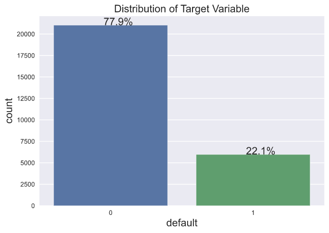
For the credit card default dataset, here is the visualization for illustrating the distribution of the target variable, which demonstrates that 22.1% of this customer base belong to the minority class. According to Google’s Machine Learning course, a dataset with 20%-40% minority class is considered mildly imbalanced, 1%-20% as moderately imbalanced, and anything less than 1% as extremely imbalanced.
Code for Displaying Imbalanced Distribution
To run the code, you will need to import the dataset and perform a 80/20 training-validation split. I opted not to do any preprocessing or feature engineering before training the model.
Why do we need to address the imbalance to begin with?
Imbalanced datasets present a challenge to the data scientist because most of the machine learning algorithms are expecting a balanced class distribution and perform optimally with such a distribution. With an overrepresentation of one class, the model will be biased towards that majority class and treat the minority class as mere noise in the data. The metrics we have relied on as our standard bearers such as accuracy become moot and meaningless.
Let’s imagine a scenario where we have a dataset of 10,000 customers with 9,500 non-defaulters and 500 defaulters, and we have identified 9250 correctly as non-defaulters (True Negatives), 25 correctly as defaulters (True Positives), 475 incorrectly as non-defaulters (False Negatives), and 250 incorrectly as defaulters (False Positives). We may be tempted to rest on our laurels with a model clocking a 92.75% accuracy, but upon closer inspection, despite such a high accuracy, our model was only able to identify a mere 25 out of the 500 minority cases. If we solely relied accuracy as our performance metric, we would be poorly misled into believing that our model was able to properly predict defaulters. If we were trying to identify patients testing positive for cancer, we realize the potentially negative ramifications of not being able to identify the minority class, namely those testing positive for cancer.
What are some of the tools for handling class imbalance?
- Weighting the training samples differently
- Incorporating additional datasets for more minority class instances
- Resampling the training dataset
I will only focus on the resampling methods in this blog. Admittedly, the doxology at Flatiron has biased me towards options 2 and 3 for my projects, but time did not permit me incorporating another dataset for the project.
Review of Performance Metrics
We saw earlier how accuracy provides a misleading indication of model performance so we must look to some other metrics during the training process for evaluating our model with imbalanced datasets. So let’s take a look at the metrics I used in evaluating my models:
Precision and Recall
If we take a look at the formula for precision, which is (TP / TP + FP), and for recall, which is (TP / TP + FN), we will notice that these two metrics notably ignores True Negatives. Precision tells us out of all the positives we predicted to be positive (i.e. the TP’s and FP’s) what percentage did we predict correctly and are truly positive. Recall (or TPR) tells us instead out of the total positive instances (i.e. the TP’s and FN’s) how many of these did we predicted as positive as a percentage.
If we look more closely at the two formulas, a model that minimizes false positives will have an increasing precision, and a model that minimizes false negatives an increasing recall. As the FP’s approaches zero, precision becomes closer and closer to simplifying to the fraction TP/TP, in other words, approaches one. Similarly, as the FN’s approaches zero, recall approaches one.
From the above scenario, let’s recall that the number of TP’s was 25, FP’s 250, and FN’s 475, which gives us a precision of 9% and recall of 5%, which does not bode well for identifying defaulters. This stresses the importance of looking at metrics other than accuracy.
F1 Score
This is the harmonic mean of recall and precision, so it takes both false positive and false negatives into account. Since we want to minimize both FP’s and FN’s, maximizing the F1 score would be a useful metric in selecting the best model. Just like with bias and variance, recall and precision have a similar interplay, where improving one comes at the cost of the other.
ROC Curve and ROC-AUC Score
This is the metric most often used to compare different models for imbalanced datasets instead of accuracy. It plots the FPR on the x-axis and TPR on the y-axis. TPR (or recall) is out of the positive class how many did we predict correctly, while FPR is out of the negative class (FP’s and TN’s) how many did we predict incorrectly. So here we have a situation where we want to maximize one and minimize the other, namely maximize TPR and minimize FPR.
It is worth noting that a baseline model with an ROC-AUC score of 0.5 indicates that this classifier has no discriminative power whatsoever, which would correspond to the diagonal line from the lower left to upper right in the metric plot. This could be one of two scenarios, either the model is predicting random or constant class for every data point. That is to say, for instance, at the upper right corner, where TPR and FPR are both equal to 1, while every member of the positive class was classified correctly, everyone in the negative class was classified incorrectly.
Until recently, I hadn’t put much thought into what a ROC-AUC score of 0 would mean, but that would mean that all the positive class instances were predicted as negative and all of the negative as positive. When AUC is between 0.5 and 1, our model is able to detect more TP’s and TN’s than FN’s and FP’s, hence able to distinguish between the positive and negative classes better.
PR Curve and PR-AUC Score
The PR-curve plots recall on the x-axis and precision on the y-axis. The baseline is dependent on the distribution of the dataset. For a perfectly distributed dataset, baseline is at 50%. A random estimator would have a PR-AUC score equal to the percentage of positive instances in the dataset. For a dataset with 10% positive instances, the baseline PR-AUC score is 0.10, so a number above that baseline would constitute an improvement on the score. For our current dataset, the baseline PR-AUC score would be about 0.22.
While I used PR-AUC as a metric during the project, since then my understanding is that it is more useful in highly imbalanced datasets or when comparing models with similar extreme imbalance.
Code for Evaluating Model Performance
Overview of Resampling Methods
For resampling the training dataset, the module imbalanced-learn provides four different categories of methods or techniques for the task at hand:
- Undersampling methods
- Oversampling methods
- Combined methods
- Ensemble methods
Here’s a quick review of the different categories since a comprehensive discussion would be a blog post in itself. Undersampling involves removing instances from the majority class, oversampling involves adding instances of the minority class, and combination methods resample both classes all with the goal to create a more even distribution of the two classes. I think this was drilled into our heads at Flatiron that oversampling is used more preferably than undersampling since we could be losing important information through the latter. However, the former has its own pitfalls, which includes the potential for replicating uninformative instances.
Undersampling methods fall under two categories: fixed and cleaning under sampling. Fixed undersampling methods are those that remove minority instances until the dataset is balanced, while cleaning methods clean the feature space based on some criteria or algorithm with Of the methods we have implemented, One Sided Selection, Edited Nearest Neighbours, and Tomek Links would be considered cleaning methods, while Near Miss would be considered fixed if you look at the distribution of the majority and minority class after resampling.
Oversampling methods include techniques that either duplicate minority instances, such as Random Over Sampling, or generate synthetic instances based on some algorithms, such as with SMOTE. By oversampling the minority class, our model learns the specifics of the minority class, and it is unable to generalize well. To offset this tendency to overfit, SMOTE randomly generates a new sample along the line segment in feature space that connects two neighboring minority instances. Ultimately, it has become one of the favored methods for oversampling to beget a whole family of SMOTE variants.
Speaking of which, combined methods bring together the best of both worlds in an attempt to address the drawbacks of SMOTE, which include its tendency to create additional noise and overlapping classes through its blind selection of nearest neighbors. ENN and Tomek Links are each implemented subsequent to the SMOTE process as a filtering means to mitigate some of the drawbacks.
Lastly, ensemble methods fall under two main categories: boosting and bagging. Boosting involves training the classifiers in sequence or series with all training samples weighted equally, and after each iteration the weights are increased on those the model misclassified. Bagging or bootstrap aggregation involves fitting the base classifier on subsets of the original dataset and then aggregating the predictions through averaging or voting.
Code for Model Training
We want to run a classifier DummyClassifier() with the following parameter strategy=most_frequent to determine our baseline scores. So what does that mean? The classifier predicts the most frequent label in the training set, i.e. predicts 0 or the majority class for every single instance. Given that scenario, what would be our accuracy? We would get an accuracy equal to the proportion of the majority class or 78.12%.
As for the PR-AUC score, it would be equal to the proportion of the minority class (21.88%), and for ROC-AUC, it should be equal to 0.5, which corresponds to having no discriminative power as we established earlier.
Below is the code to run the oversampling method of SMOTE, but we would instantiate a different resampling method, but run the run_resampling function plugging in the new method. This can be applied for all undersampling, oversampling, and combined resampling methods.
Just as a reminder, we performed a 80/20 split on the dataset, split feature (X) variables from the target (y) variable, run fit_transform on the training (X_train) set and just transform on the testing set (X_valid). Several models were run on the training data, and the best model was determined prior to resampling. Because we are jumping in mid-process, that is how we arrived at GradientBoostingClassifier() in the code.
We normalized the dataset with StandardScaler(), but as a reminder we want to run .fit() and .transform() on the training set, but only .transform() on the testing or validation set. That would be X_train_norm and X_valid_norm in the above function.
Final Thoughts on Original Project
I was originally hesitant to summarize my results for my Phase 3 project since I had anticipated that resampling would have produced some substantive change in metrics. None of them produced an accuracy that was greater than the base classifier, but Tomek Links and One-Sided Selection were the closest. SMOTE produced a higher F1 score at the cost of accuracy, while Tomek Links has a similar accuracy with a slightly improved F1 score. I was unable to improve on the PR-AUC or ROC-AUC score, which essentially remained static throughout.
Ultimately, in my project, through fine-tuning the hyperparameters, I was able to push my accuracy and ROC-AUC scores higher.
Here is the dataframe of the metrics from my original project:
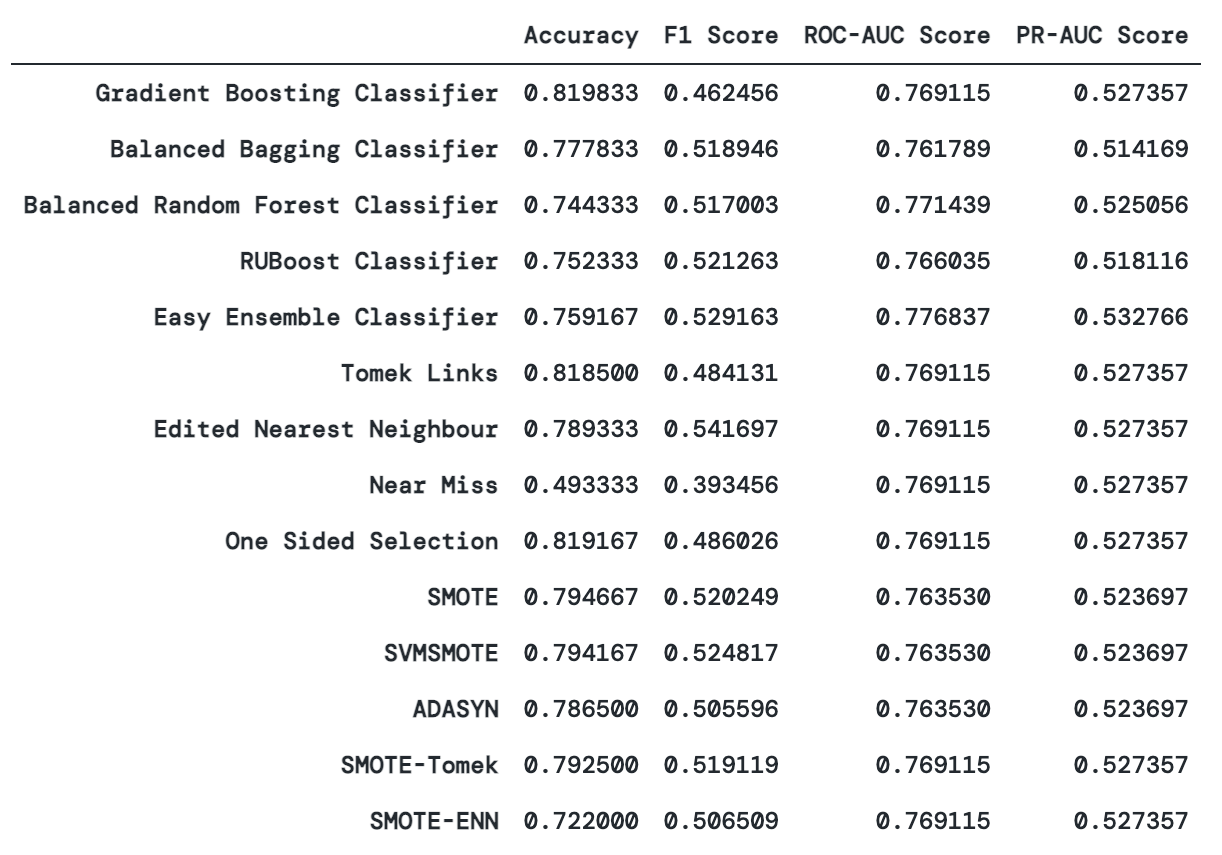
In retrospect, with a baseline accuracy of 78%, I still think there is room for potential improvement. I would have tolerated a decrease in accuracy for an increase in ROC-AUC or F1 score.
In the grand scheme of imbalanced datasets, I would consider this dataset as only mildly imbalanced, and as such resampling methods may not be as effective perhaps even detrimental towards them. Upon reviewing some of the Kaggle repos, it seems that my struggles in improving the accuracy and ROC-AUC score is not without precedent. However, this is worth further investigation since Alam et al. produced a 89% accuracy with a GBDT model using K-Means SMOTE oversampling, and Islam et al. produced a 95% accuracy with their Machine Learning Approach.
The code for the blog is a simplified version of my original project, which is located here:
Resources:
Google’s Machine Learning Crash Course: https://developers.google.com/machine-learning/crash-course
User Guide for imbalanced-learn: https://imbalanced-learn.org/stable/user_guide.html
Natalie Hockham: Machine learning with imbalanced data sets: https://www.youtube.com/watch?v=X9MZtvvQDR4
References:
Alam, T.M., Shaukat, K., Hameed, I., Luo, S., Sarwar, M.U., Shabbir, S., Li, J., & Khushi, M. (2020). An Investigation of Credit Card Default Prediction in the Imbalanced Datasets. IEEE Access, 8, 201173–201198. https://doi.org/10.1109/ACCESS.2020.3033784
Ma, Y. (2020). Prediction of Default Probability of Credit-Card Bills. Open Journal of Business and Management, 08, 231–244. https://doi.org/10.4236/ojbm.2020.81014
Torrent, N.L., Visani, G., & Bagli, E. (2020). PSD2 Explainable AI Model for Credit Scoring. ArXiv, abs/2011.10367. https://arxiv.org/pdf/2011.10367.pdf
Lemaître, G., Nogueira, F., & Aridas, C.K. (2017). Imbalanced-learn: A Python Toolbox to Tackle the Curse of Imbalanced Datasets in Machine Learning. ArXiv, abs/1609.06570. https://jmlr.org/papers/v18/16-365.html
Galar, M., Fernández, A., Tartas, E., Bustince, H., & Herrera, F. (2012). A Review on Ensembles for the Class Imbalance Problem: Bagging-, Boosting-, and Hybrid-Based Approaches. IEEE Transactions on Systems, Man, and Cybernetics, Part C (Applications and Reviews), 42, 463–484. https://doi.org/10.1109/TSMCC.2011.2161285
García, V., Sánchez, J., & Mollineda, R.A. (2010). Exploring the Performance of Resampling Strategies for the Class Imbalance Problem. IEA/AIE. https://doi.org/10.1007/978-3-642-13022-954
Islam, S.R., Eberle, W., & Ghafoor, S. (2018). Credit Default Mining Using Combined Machine Learning and Heuristic Approach. ArXiv, abs/1807.01176. https://arxiv.org/pdf/1807.01176.pdf

