


1. INTRODUCTION
The Admiralty Manual of Navigation 1938, p166 states
In the practice of navigation, when a cocked hat is obtained, it is customary to place the ship's position on a chart in the most dangerous position that can be derived from the observations because the existence of a cocked hat is evidence that the observations are inaccurate, and by interpreting them to his apparent disadvantage, the navigator gives himself a margin for safety which he might not otherwise have.
and in practice this is often interpreted as choosing the vertex of the cocked hat closest to danger. Under the assumption that the errors in the intercepts are normal, independent and identically distributed with mean zero, the contours of the probability distribution of the position, given the lines of position, are curves such that the sum of the squared distance from each of the lines is constant. These form a family of concentric ellipses. Under these assumptions one might interpret the above advice in the following way: “choose a contour according to your appetite for risk and assume your position is the closest point on that contour to danger”. One can of course calculate the family of elliptical contours algebraically, but in this paper we identify them as intrinsic properties of the angles between the lines and from this we hope to gain some further insight into the dependence of the probability contours on the position lines. The most probable position can be constructed by ruler and compasses in a simple and intuitive manner. Any point is constructible if it can be expressed in terms of known lengths using the basic operations of arithmetic together with the square root, (Stewart, Reference Stewart2015). Practically the methods for operations such bisecting an angle and constructing a perpendicular bisector are given in elementary texts on geometric and mechanical drawing such as (Morling, Reference Morling2010). So for a given sum of squared distance the centre, vertices, axes, foci,; of the ellipse are also constructible by following the arithmetic steps of the matrix operations, including finding eigenvalues. However giving a geometric description means that we have a much simpler and intuitive construction using operations, such as bisection of angles and constructing perpendicular bisectors of line segments, familiar in traditional navigation. We hope it will also help the navigator to understand better the dependence of the probability contours on the angles between the lines of position and the variances of the errors.
The obvious traditional application to navigation is the case of (nearly) simultaneous observation of the altitudes of three celestial bodies with known azimuths. We use the plane approximation to the Earth's surface near the assumed position, and assume the azimuths are known exactly. After averaging several observations for each body we make the assumption that the errors in the intercepts are normally distributed with mean zero and the same variance σ2. A wide variety of positioning methods over scales ranging from oceans to rooms rely on lines of position, whether they be straight line approximations to curves from a constant distance to a point, or difference in distances from two points, or bearings taken of known landmarks or from a number of fixed stations. Dead-reckoning and inertial navigation methods continue to develop apace, and these can be augmented by lines of position from a distance or bearing. The errors of such methods accumulate over time and often will be direction-dependent. For example distance run and cross-track errors might have different variances. Nevertheless they can be expressed as lines of position with a known variance (in the parallel displacement) and incorporated into the same mathematical framework as lines derived from bearings or distances.
Lines of position that are bearings from known locations, even if the angular errors are identical in each bearing and the objects assumed distant, result in lines of position with a standard deviation proportional to the distance to the object. For a through treatment of this case see (Stansfield, Reference Stansfield1947), who includes the case of more than three lines of position and many examples of ellipses for the case of three lines, although the examples are calculated numerically.
In this paper we assume systematic errors, such as index error in a sextant, have been removed by calibration, leaving only random errors with zero mean. In celestial navigation these include the error in judging the coincidence of the star or planet, or the limb of the Sun or Moon, and the horizon, Gordon (Reference Gordon1964) analysed the contribution of the sea state (for a small vessel) and the visibility of the horizon. In reading the vernier on the drum there is at least a rounding error as well as a possibility of misreading the vernier scale. There may also be errors in recording the time of the sight. Especially for bodies at lower altitudes, errors may be caused by variability in the refractive index of the atmosphere, (Peterson, Reference Peterson1952), (Fletcher, Reference Fletcher1952). Regression techniques (in most cases linear regression) can be used for a series of sights of the same body. This results in an improvement in the accuracy and an estimate of the variance (Burch and Miller, Reference Burch and Miller2014). In (Shufeldt, Reference Shufeldt1962) a careful study was carried out of the precision of sextant measurements and one of the conclusions was that “only a small number [of people] have the ability of judging the instant of contact between the body and the horizon.” That paper also notes that the Nautical Almanac only gives the precision required for a position fix with an accuracy up to 0·2 nautical miles. Of course if greater precision is needed ephemeris and correction calculations can now be performed with greater accuracy using a small computer, but the skill of the observer and the motion of the vessel will always limit the accuracy of the observations.
2. ALGEBRAIC FORMULATION
For simplicity we begin with three lines of position, with equal variances. We will assume that the normally distributed error results in a parallel translation of the lines while the direction of the lines is assumed to be correct. Let θi, i=1, 2, 3 be the angles normal to the lines of position make to the x 1 (traditionally East) Cartesian axis. In the case of a fix in celestial navigation, lines of position are normal to the azimuth Z i of the celestial body, so θi, in degrees, is 90° − Z i.
The equations for the lines of position are x 1cosθi + x 2sinθi = d i, an overdetermined system of equations denoted in matrix form as Nx = d where
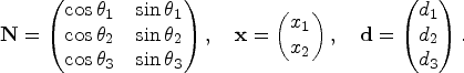 $$\mathbf{N}=\left(\begin{matrix} \cos \theta_1 & \sin \theta_1\\ \cos \theta_2 & \sin \theta_2 \\ \cos \theta_3 & \sin \theta_3 \\ \end{matrix} \right),\quad \mathbf{x}=\left(\begin{matrix} x_1 \\ x_2 \end{matrix}\right),\quad \mathbf{d}=\left(\begin{matrix} d_1 \\ d_2 \\ d_3 \end{matrix}\right).$$
Here N is the matrix whose columns are normal vectors to the lines of position (see Figure 1) while d is the vector of the distances between the lines of position and the origin, while x is the position vector of a location under consideration. The system is inconsistent with probability one. However, one might encounter the situation in which the triangle, or “cocked hat”, is small despite large errors. The Admiralty manual is right to take a large cocked hat as a symptom of large errors, but one cannot be sure the errors are small because we have a small cocked hat.

Figure 1. Three coincident lines of position (LOP) enclosing the cocked hat, normal vectors labelled N i (rows of N). The symmedian point, labelled K, minimises the sum of the squared distance to the lines.
Assuming Gaussian errors in d the joint probability density function for the position x is proportional to
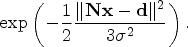 $$\exp\left( -\frac{1}{2}\frac{\|\mathbf{N} \mathbf{x} -\mathbf{d} \|^2}{ 3 \sigma^2}\right).$$
The point that maximises the probability, called the Most Probable Position in the navigation literature and the Maximum Likelihood Estimate in statistics, minimises  $\|\mathbf{N} \mathbf{x} -\mathbf{d}\|^{2}$ and is given by
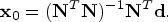 $$\mathbf{x}_0 = (\mathbf{N}^T\mathbf{N})^{-1}\mathbf{N}^T \mathbf{d}.$$
Even without the Gaussian assumption, provided the errors in each line have mean zero, are uncorrelated and with equal variance, x0 is still the best linear unbiased estimator, according to the Gauss-Markov theorem, (Björck, 2015, Thm 2.1.1). The matrix applied to d in (3), is known as the Moore-Penrose generalised inverse of N, (Björck, 2015, p230). For simplicity let us now move the origin of our Cartesian coordinate system to x0, which means d becomes d − Nx0. The new d is in the orthogonal complement to the range of N, that is the null space of NT. In the new coordinates the probability contours are given by
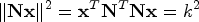 $$\Vert \mathbf{N} \mathbf{x}\Vert^2 =\mathbf{x}^T \mathbf{N}^T\mathbf{N}\mathbf{x}= k^2$$
for constant k.
We can calculate (compare (Stansfield, Reference Stansfield1947, equations (8)), and (Stuart, Reference Stuart2019, Appendix C))
 $$\mathbf{N}^T\mathbf{N}= \frac{1}{2} \left( 3 I + \left(\begin{matrix} \displaystyle\sum_{i=1}^3\cos 2 \theta_i & \displaystyle\sum_{i=1}^3\sin 2 \theta_i \\ \displaystyle\sum_{i=1}^3\sin 2 \theta_i& -\displaystyle\sum_{i=1}^3\cos2 \theta_i \\ \end{matrix} \right) \right).$$
Let  $\Gamma= \sum_{i < j} \cos 2 ( \theta_{i}-\theta_{j}) $; then
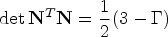 $$ \det \mathbf{N}^T\mathbf{N} =\frac{1}{2} ( 3-\Gamma)$$
and
 $$ \mathrm{tr} \mathbf{N}^T\mathbf{N} = 3.$$
So the eigenvalues are  $\lambda_{1,2} = \frac{1}{2} \left(3\pm \sqrt{3 + 2 \Gamma}\right)$, and these are the reciprocal squares of the lengths of the semi-major and semi minor axes. Note that Γ is a symmetric function of the exterior angles of the triangle so is a similarity invariant. A pair of eigenvectors of NTN, vi give the directions of the major and minor axes respectively
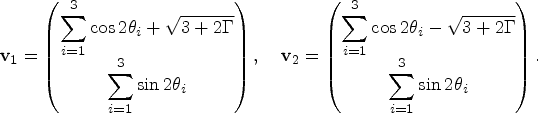 $$\mathbf{v}_1=\left( \begin{array}{@{}c@{}} \displaystyle\sum_{i=1}^3\cos 2 \theta_i + \sqrt{3 + 2 \Gamma}\\ \displaystyle\sum_{i=1}^3\sin 2 \theta_i\\ \end{array} \right),\quad \mathbf{v}_2=\left( \begin{array}{@{}c@{}} \displaystyle\sum_{i=1}^3\cos 2 \theta_i - \sqrt{3 + 2 \Gamma} \\ \displaystyle\sum_{i=1}^3\sin 2 \theta_i\\ \end{array} \right).$$
From the singular value decomposition of N (Golub and Van Loan, 1996, p20) we note that ui = Nvi are eigenvectors of NNT with the same eigenvalues and there is a third orthogonal eigenvector u3 which spans the null space of NT. We have
 $$\mathbf{N}\mathbf{N}^T = \left( \begin{array}{ccc} 1 & \cos ( \theta_1-\theta_2) & \cos ( \theta_1-\theta_3) \\ \cos ( \theta_1-\theta_2) & 1 & \cos ( \theta_2-\theta_3) \\ \cos ( \theta_1-\theta_3) & \cos ( \theta_2-\theta_3) & 1 \\ \end{array} \right)$$
with
 $$\mathbf{u}_1 = \left( \begin{array}{@{}c@{}} \sqrt{2 \Gamma +3}+1+\cos ( 2 ( \theta_1-\theta_2) ) +\cos ( 2 ( \theta_1-\theta_3) ) \\ \left(\sqrt{2 \Gamma+3}+2\right) \cos ( \theta_1-\theta_2) +\cos ( \theta_1- \theta_3+\theta_2-\theta_3) \\ \noalign{\vskip3pt} \left(\sqrt{2 \Gamma+3}+2\right) \cos ( \theta_1-\theta_3) +\cos ( \theta_1- \theta_2+\theta_3 - \theta_2) \\ \end{array} \right),\quad \mathbf{u}_3 = \left( \begin{array}{@{}c@{}} \sin ( \theta_2-\theta_3) \\ \sin( \theta_3-\theta_1) \\ \sin ( \theta_1-\theta_2) \end{array} \right),$$
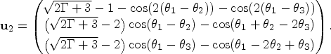 $$\mathbf{u}_2 = \left( \begin{array}{@{}c@{}} \sqrt{2 \Gamma+3}-1 -\cos( 2( \theta_1-\theta_2) ) - \cos( 2( \theta_1-\theta_3) ) \\ \left(\sqrt{2 \Gamma+3}-2\right) \cos ( \theta_1-\theta_2) -\cos ( \theta_1+\theta_2-2 \theta_3) \\ \noalign{\vskip3pt} \left(\sqrt{2 \Gamma+3}-2\right) \cos ( \theta_1-\theta_3) -\cos ( \theta_1-2 \theta_2+\theta_3) \end{array}\right).$$
We notice that the expressions for NNT and the ui can be written in terms of only trigonometric functions of the angles θi − θj, whereas for the vi this does not seem to be the case. In the case where the normals are all either pointing out of the triangle or in to the triangle |θi − θj| are the exterior angles (supplements of the interior angles) of the triangle. We seek to understand how the axes depend on the shape of the triangle, and to describe them in a way that is independent of rotations and scaling of the coordinate system. The lack of symmetry between the components of the eigenvectors ui is inconvenient and we find a more symmetrical representation in Section 4. A ruler and compasses construction for the solution to (3) is given in (Coolidge, Reference Coolidge1913), for the case of n>2 lines, however it involves graphically forming sums of trigonemetric functions of θi and seems rather laborious.
3. GEOMETRY OF TRIANGLES
First we introduce a system of homogeneous coordinates relative to the triangle. Let A, B, C and P be points in a plane. Consider the triangle ABC and α, β, and γ the signed distances between P and the side lines BC, CA, AB of the triangle; then (ℓα, ℓβ, ℓγ) are trilinear coordinates, (Whitworth, Reference Whitworth1866), of P for any non-zero ℓ. Three points P 1, P 2, P 3 are collinear if and only if their trilinear coordinates satisfy
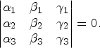 $$\left\vert \begin{array}{@{}ccc@{}} \alpha_1 & \beta_1&\gamma_1\\ \alpha_2 &\beta_2 &\gamma_2\\ \alpha_3 &\beta_3 &\gamma_3 \end{array} \right\vert =0.$$
In trilinear coordinates the incentre (centre of inscribing circle) is given by (1, 1, 1) the circumcentre (centre of circumscribing circle) by (cos A, cos B, cos C) in terms of the interior angles at the vertices, or
 $$( a(b^2 + c^2 - a^2), b(c^2 + a^2 - b^2), c(a^2 + b^2 - c^2) )$$
in terms of the side lengths a, b and c. We note that for all these centres the trilinear coordinates can be written as (f(a, b, c), f(b, c, a), f(c, a, b)) where f is a homogeneous function of three variables with f(a, b, c) = f(a, c, b). This has been generalised so any point with trilinear coordinates that can be expressed in this way is called a triangle centre (although it need no longer lie inside the triangle), see (Kimberling, Reference Kimberling1994). The triangle centres with known interesting properties are listed in a catalogue, The Encyclopedia of Triangle Centers (ETC), (Kimberling, Reference Kimberling2018), and the centres designated by X(i) for a positive integer i; more examples are given in Table 1 and Figure 2.
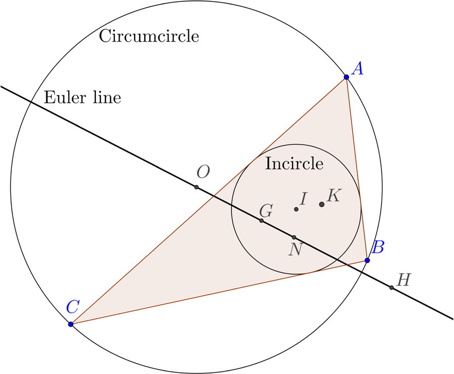
Figure 2. Triangle centres (see Table 1), circumcircle, incircle and Euler line plotted using Geogebra, (Hohenwarter, Reference Hohenwarter2018).
Table 1. Table of triangle centres with their trilinear coordinates and number in the Encyclopedia of Triangle Centres, (Kimberling, Reference Kimberling2018). The angles at the vertices are denoted by A, B, C and the side lengths opposite these vertices by a,b,c.

In our problem, for a point x in the plane, Nx − d is exactly a vector of signed distances from the lines of position, the side lines of the cocked hat. We can choose the normal directions θi (by possibly adding 180°) so that the normals defined by the rows of the matrix N point towards the interior of the triangle, so that the vectors of signed distances are trilinear coordinates. See Figure 1. We see immediately that the null vectors of NT are exactly those that result in the zero solution, and our origin is at the symmedian point (also called the Lemoine point), for which sines of exterior angles are trilinear coordinates. This is another way of explaining the original derivation of the symmedian point as the solution to this problem in navigation (Yvon-Villarceau and Aved de Magnac, Reference Yvon-Villarceau and Aved de Magnac1877). Yvon-Villarceau gave the trilinear coordinates of the symmedian point in terms of the side lengths as (a, b, c). We see from Table 1 that the trilinear coordinates of triangle centres can be given in terms of lengths or interior angles. The sine rule
 $$\frac{a}{\sin A} =\frac{b}{\sin B}=\frac{c}{\sin C}= 2R,$$
where R is the circumradius, gives a simple way to convert between the two. As an example of their use consider a triangle ABC with a right angle at C. From the expression for the trilinear coordinates we see that the distances between the symmedian point K and the sides are in the ratio a:b:c, where a 2+b 2=c 2. It is easy to see from this that the symmedian point lies on the altitude (the line from a vertex perpendicular to the opposite side) to the hypotenuse. For a proof see (Honsberger, Reference Honsberger1995, p59).
4. AXES OF THE ELLIPSES
As Nvi is a scalar multiple of ui, i=1, 2 we can take our expressions for these as trilinear coordinates for a point on the major and minor axes. As we know the axes pass through the symmedian point we see that the equations for the trilinear coordinates of the axes are Ui · (α, β, γ)T = 0 where Ui = ui × u3. While our expressions for the ui, i=1, 2 are in terms of exterior angles of the triangle the components are not all the same function subjected to a permutation. We therefore seek a triangle centre in the ETC that lies on the same line.
The centres X(1344) and X(1345), internal and external centre of similitude of circumcircle and orthocentroidal circle (see Figure 5 for construction), are given in trilinear coordinates in terms of J, see Table 2, where
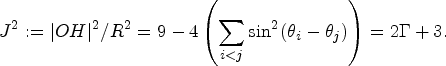 $$J^2:=|OH|^2/R^2 = 9 -4\left( \sum_{i< j} \sin^2 (\theta_i-\theta_j)\right)=2 \Gamma +3.$$
Table 2. Further triangle centres used in this paper with their trilinear coordinates. Here only the first component of the coordinates is given while the others are obtained by cyclic permutations of the angles A,B,C. Here J = |OH|/R where R is the circumradius and |OH| the distance between the circumcentre and orthocentre.

Here |OH| is the distance between the circumcentre and the orthocentre. So in terms of J the eigenvalues are (3±J)/2, and the eccentricity  $e = \sqrt{1 - \lambda_{2}/\lambda_{1}}= \sqrt {2 J/(3+J)}$.
To show that u1 lies on the line defined by X(6) and X(1344) we calculate the determinant |u1, u3, X(1345)| = U1 · X(1344), using the notation αij = θi − θj
 $$\begin{align}&\left\vert \begin{matrix} \sin \alpha_{23} & \sin \alpha_{31}\\ J+1+\cos 2 \alpha_{12} +\cos 2 \alpha_{13} & ( J+2) \cos( \alpha_{12}) +\cos ( \alpha_{13} +\alpha_{23}) \\ ( 1-J) \cos \alpha_{23} -4 \cos\alpha_{12} \cos \alpha_{13}& ( 1-J) \cos ( \alpha_{13}) -4 \cos\alpha_{12}\cos\alpha_{23} \end{matrix}\right.\notag\\ &\quad \left.\begin{matrix} \sin \alpha_{12} \\ ( J+2) \cos \alpha_{13} +\cos ( \alpha_{12} +\alpha_{32}) \\ ( 1-J) \cos \alpha_{12}-4 \cos\alpha_{13}\cos \alpha_{23} \end{matrix}\right\vert=0 \end{align}$$
by application of sum and product formulae for trigonometric functions. Similarly we see that the eigenvector associated with the minor axis lies on the line defined by X(6) and X(1345).
The equation for the line through X(6) and X(1344), the major axis, is given in trilinear coordinates (x, y, z) by
 $$\begin{align} & x \sin ( \alpha_{21} + \alpha_{31} ) ( 2 \cos 2 \alpha_{23}-J+1) + y \sin ( \alpha_{12}+\alpha_{32}) ( 2 \cos 2\alpha_{13}-J+1) \notag\\ &\quad + z \sin ( \alpha_{13}+\alpha_{23}) ( 2 \cos 2 \alpha_{12} -J+1) =0.\label{eq14} \end{align}$$
In terms of interior angles the major axis is
 $$\sin(B-C)(2 \cos 2A -J+1)x + \mbox{(cyclic)} =0$$
where the other two terms in y and z are formed by cyclic permutations of A, B, C, while the minor axis is
 $$\sin(B-C)(2 \cos 2A +J+1)x + \mbox{(cyclic)} =0.$$
5. FURTHER GEOMETRIC PROPERTIES
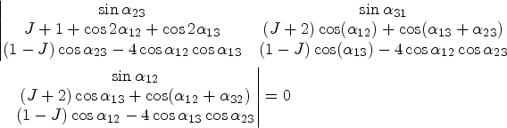
The medians are the lines connecting a vertex of the triangle to the midpoints of the opposite sides and these three lines intersect at the centroid. The angle bisectors also intersect, at the incentre. The symmedian lines are formed by reflecting the medians in the angle bisectors, and the symmedian lines intersect at the symmedian point; see Figure 3.
Figure 3. Construction of symmedian lines and point. Given triangle ABC the medians CE and BG join a vertex to the midpoint of the opposite side. The bisectors of the vertex angles are CD and BF and the symmedian lines BG′ and CE′ are the reflections of the medians in the angle bisectors and meet at the symmedian point K. The construction gives the same point regardless of which pair of vertices is used.
Clearly these constructions can all be done fairly swiftly with a straight edge and pair of compasses. For the case of non-equal variances, it is interesting to note that (Stansfield, Reference Stansfield1947, Fig. 8) defines what could be thought of as weighted symmedian lines and a weighted symmedian point. This is analogous to the centre of mass when three different masses are placed at the vertices of the triangle: a weighted centroid. We explore this further in Section 9.
We now consider possible constructions for the axes. The Euler line for any non-equilateral triangle passes through the circumcentre X(3), orthocentre X(4), the centroid X(2), and nine-point centre X(5). It passes through the centre of the circumcircle and intersects the circle at two points X(1113) and X(1114), (Moses and Kimberling, Reference Moses and Kimberling2007).
The Simson line, (Coxeter and Greitzer, Reference Coxeter and Greitzer1967), of a point P on the circumcircle is the line that passes through the closest approaches of the side lines to P. Our axes are parallel to the Simson lines of X(1113) and X(1114) and pass through the symmedian point. See Figure 4. For a proof see (Bilo, Reference Bilo1987).
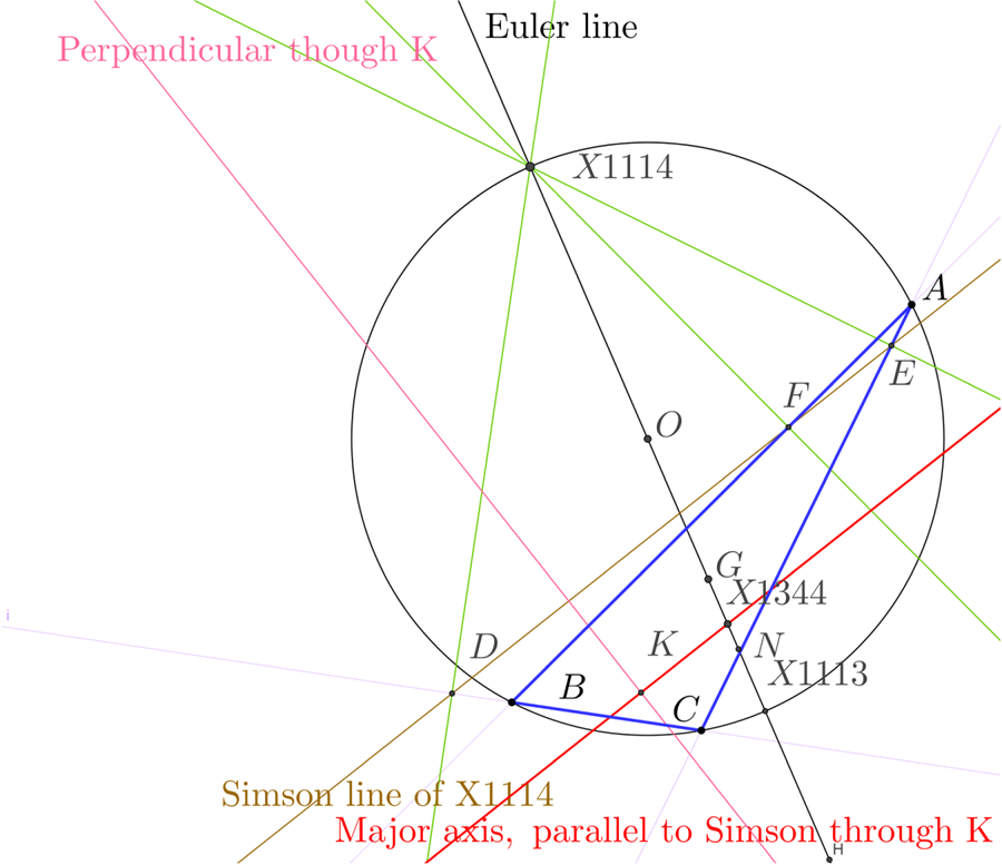
Figure 4. The construction of the axes using the Simson Line. X(1114) is the intersection of the Euler line with the circumcircle and its Simson line DFE passes through the feet of the perpendiculars to the side lines through X(1114). The major axis (in red) is the line parallel to this through the symmedian point K.
An alternative construction is to first construct X(1344) and X(1345). The orthocentric circle is the circle with the orthocentre and centroid as a diameter. Given two circles, the centres of similitude are constructed using parallel diameters on the two circles and then joining the intersection of the diameters with the circles across the two circles. There are two ways to do this taking the points on the opposite and same side of the line joining the centres of the circles. These are the internal and external centres of similitude. The internal and external centres of similitude of the orthocentric and circumcentric circles are X(1344) and X(1345). The axes are the lines joining these points respectively to the symmedian point. See Figure 5.

Figure 5. Construction of centres of similitude of the orthocentric circle and the circumcircle. Any diameter of the circumcircle FOF′ is chosen. The orthocentric circle is the circle with GH as a diameter, but a diameter EE′ is drawn parallel to FOF′. Line FE meets F′E′ at X(1345), while EF′ meets FE′ at X(1344).
The semi-major axes are convenient as the ellipse lies between circles with these as radii centred on the centre of the ellipse. Given X(3) and X(4) we have line-segments with length |OH| and R and hence we can construct the ratio of the eigenvalues. If we choose a point on the major axis we can now find the corresponding point on the minor axis for that value of k.
Notice that the shape of the family of ellipses and the orientation of the axes is determined by the azimuths of the lines independent of the size of the cocked hat.
6. ANGLE BETWEEN MAJOR AXIS AND SIDE OF TRIANGLE
We would like to understand the alignment of the axes relative to the sides of the triangle. There is a formula given in (Whitworth, Reference Whitworth1866, p50) for the tangent of the angle between two lines in trilinear coordinates. Applying this to the major axis and the line BC, and denoting the angle by ϕBC gives
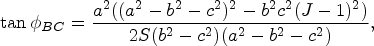 $$\tan \phi_{BC}=\frac{a^2 ((a^2 - b^2 - c^2)^2 - b^2 c^2 (J - 1)^2)}{2 S (b^2 - c^2) (a^2 - b^2 - c^2)},$$
where S is twice the area of the triangle. In terms of interior angles at the vertices and using double angle trigonometric formulae, the tangent of twice the angle between the major axis and B can be written as
 $$\tan 2 \phi_{BC}=\frac{2 \cos A \sin(B - C)}{ 2 \cos A \cos(B - C) - 1} =\frac{ 2 \sin (B - C) }{ 2 \cos (B - C) - \sec A},$$
which is seen to be zero for a right triangle having A=π/2, the major axis parallel to the hypotenuse. For an isosceles triangle having B=C we also have zero but for A<π/2, an acute isosceles triangle the angle is π/2 whereas for the obtuse case it is zero, taking account of the ambiguity in the inverse tangent. For B≠C as A approaches π, we have BC the longest side, |B−C|<B+C must tend to zero as B and C tend to zero, again giving the major axis approaching the same direction as BC.
These formulae are invariant: they not referred to a coordinate system but are given in terms of side lengths or angles of the triangle. In general a 2×2 symmetric matrix with distinct non-zero eigenvalues
 $$\begin{bmatrix} a_{11} & a_{12} \\ a_{12} & a _{22} \end{bmatrix}$$
has an eigenvector making an angle ϕ1 to the x 1 axis with
 $$\tan 2 \phi_1 = \frac{2 a_{12}}{ a_{22} - a_{11} }$$
which we can apply to NTN giving a non-invariant formula for the direction of the axis of the ellipse, indeed this is the formula used by (Stansfield, Reference Stansfield1947, Eq (12)), in the case of any number of lines of position with possibly different variances.
7. DRAWING AN ELLIPSE
An ellipse with a given centre is determined by three parameters, for example the direction of the major axis and the semi-major and semi-minor axes (that is the semi-diameters). The points where the axes meet the ellipse are called the vertices of the ellipse. While an elliptical curve cannot be drawn using only a ruler and compasses, as many points as needed on the ellipse can be. For the practical purposes of navigation drawing the axes and marking the vertices is probably enough to convey the relevant information, and given the bounding rectangle through the vertices with sides parallel to the axes an approximate ellipse drawn free hand may suffice. There are several methods taught in the context of engineering drawing to draw an approximate ellipse, (Morling, Reference Morling2010). For example in the “two circle method” circles are drawn with radii equal to the semi-axes. A diameter of the larger circle produces two points on the ellipse by intersecting lines parallel to the axes one obtains points on the ellipse. One plots as few points as are needed to join to get a smooth curve. See the example in Section 11 and Figure 16. A more mechanical method is simply to pin a piece of string at the foci, with the length adjusted so that when pulled taut it meets a vertex. A pencil is inserted in the string and the locus as it moves with the string taut is the desired ellipse.
We can construct the symmedian point as the centre of the ellipse and to methods to find an axis (and then the other is perpendicular). We can easily construct the lengths |OH| and R and so their ratio J, but given the axes there is a simpler way to draw a representative ellipse from the family. Let ψ be the angle the diagonal of the bounding rectangle to the ellipse makes with the major axis. As in Figure 5 let G be the centroid and O the circumcentre. Draw a perpendicular to the Euler line OG through G. This line intersects the circumcircle. Call one of the intersections L. Then  $\psi= \angle GOL/2$. We can either bisect ∠ GOL or simply measure it with a protractor and halve it. See Figures 15 and 16. Given the symmedian point K and X(1344) on the major axis draw a line through K at the angle ψ and this is the diagonal of the rectangle. This is enough for the two circle method to be used to plot a few points on the ellipse. If the foci are needed, one simply sets the compasses to the semi-major axis then puts the point at a vertex on the minor axis. Striking off this distance on the major axis gives the foci.
8. EXAMPLES OF ELLIPSES FOR THREE LINES OF POSITION WITH EQUAL VARIANCES
To illustrate the orientation and eccentricity of the ellipses, several examples were plotted using Geogebra for a fixed k. See Figure 6. As one expects, the eccentricity increases with the aspect ratio of the triangle with nearly circular contours for triangles close to equilateral. Indeed this is expected as the orthocentre and circumcentre are close so J is small. As we have seen in Section 6, for an isosceles triangle, if it is acute, the major axis will be aligned with the axis of symmetry, as will the minor axis if the triangle is obtuse. For a right angled triangle the circumcircle is centred on the midpoint of the hypotenuse and passes through the right angle vertex. The orthocentre also passes through the right angle vertex and X(1345) lies at this vertex. As the symmedian line through the right angle vertex is normal to the hypotenuse, we see that it is exactly the minor axis, and the major axis is parallel to the hypotenuse.
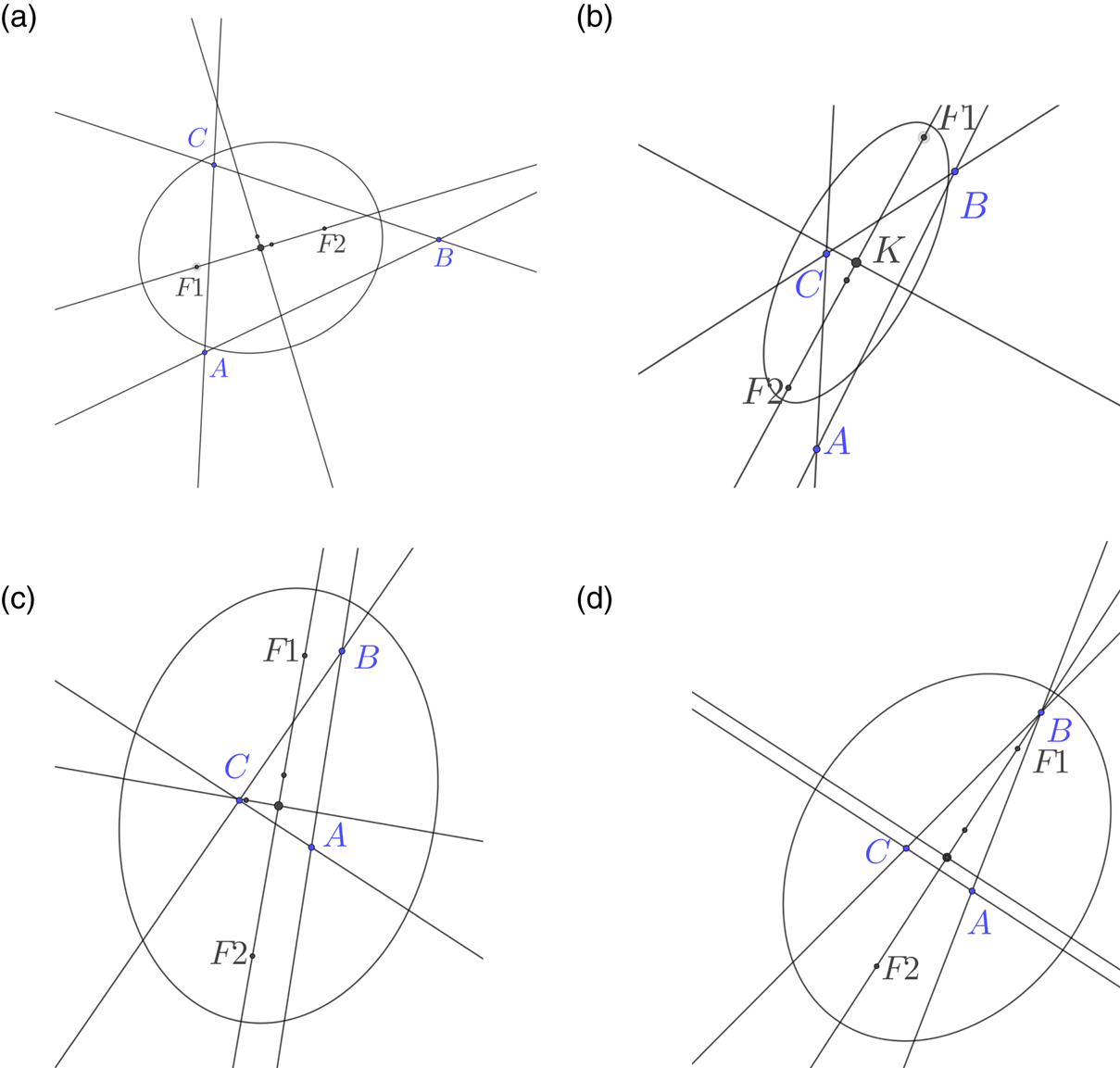
Figure 6. Ellipse shown with axes, indicating the symmedian point K, foci F1 and F2 and internal and external centres of similitude for the orthocentroidal and circumcircles X(1344) and X(1345). The major axis of the family of ellipses is aligned approximately with the longest side of the triangle. (a) The major axis is roughly aligned with the longest side. (b) Obtuse and nearly isosceles. (c) For a right angled triangle the axis is aligned with the hypotenuse (d) Acute isoceles has the major axis of the ellipse aligned with the axis of symmetry of the triangle.
9. GENERAL VARIANCES
There is a natural generalisation of the centroid of a triangle to the centre of mass of three possibly different masses at the vertices of a triangle, a weighted centroid.
In our case we continue the idea of a triangle with weights by defining w i>0 to be the reciprocal of the variance of the error in each d i, so we are concerned with the family of ellipses associated with
 $$w_1 d_1^2 + w_2 d_2^2 + w_3 d_3^2 = k^2.$$
That is
 $$(a^2k^2 -S^2 w_1) x^2 + 2 b c k^2 y z + \mbox{(cyclic)} = 0$$
in trilinear coordinates. The centre of this ellipse is the “weighted symmedian point” with trilinear coordinates (a/w 1, b/w 2, c/w 3), this being the isogonal conjugate of the weighted centroid P with trilinear coordinates (w 1/a, w 2/b, w 3/c). The axes are parallel to the Simson lines of the circumcircle intersection with the line OP, where O is still the ordinary circumcentre of the triangle ABC. To construct P notice that the line AP intersects BC at A′ where
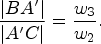 $$\frac{|BA'|}{ |A'C|} = \frac{w_3}{w_2}.$$
In a practical situation one might for example judge the error in one LOP to have twice the standard deviation of the others, and hence the ratio of the variances would be 4:1. As Stansfield (Reference Stansfield1947) argues, for LOPs’ associated bearings, if the bearings have the same accuracy, the standard deviation will be approximately proportional to the distance to the land mark.
Once P has been constructed using weights, the remaining steps can be performed with ruler and compasses
The double angle with the BC side has tangent
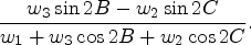 $$\frac{w_3 \sin 2 B - w_2 \sin 2 C} {w_1 + w_3 \cos 2 B + w_2 \cos 2 C}.$$
The eccentricity is
 $$\sqrt{ \frac{2 J_w }{1 + J_w}}$$
where
 $$J_w =|OP|/R = \frac{\sqrt{\begin{matrix}a^2 b^2 c^2 (w_1^2 + w_2^2 + w_3^2) + 2 a^2 (b^2 c^2 - 2 S^2) w_2 w_3\\ +\, 2 b^2 (c^2 a^2 - 2 S^2) w_3 w_1 + 2 c^2 (a^2 b^2 - 2 S^2) w_1 w_2\end{matrix}} }{ a b c (w_1 + w_2 + w_3)}$$
and we see that for w 1 large, which means LOP 1 is more reliable, the angle is smaller, and the major axis more aligned with LOP 1. If the ratios of the weights can be adjusted, for example by averaging over more readings, the question arises if there is some set of weights that make the ellipse a circle even for triangles with very different side lengths. For the weighted ellipse to be a circle we require the eccentricity to be zero in (25), and this is achieved by J w=0 in (26), which means that the weighted centroid P coincides with the circumcentre O. Referring to Table 1 we see that the trilinear coordinates of O are (cos A, cos B, cos C) so we want to make w 1/a=cos A, or w 1 = a = 2R sin A cos A = R sin 2A and cyclic permutations. We see that there is always a positive set of ratios of weights that achieve this for an acute triangle.
It is interesting to note that in the unweighed case the ellipse for a certain value of k passes through the vertices of the anti-complementary triangle to ABC. It is perhaps surprising that this is also true for the weighted case, for the value of k such that
 $$k^2 = S^2 (w_1/a^2 + w_2/b^2 + w_3/c^2).$$
10. EXTENSION TO MORE THAN THREE LINES OF POSITION
For n>3 lines of position in the plane the equation NTN, (4), holds when 3 is replaced by n (c.f. (Stansfield, Reference Stansfield1947)). The analogous expression for NNT to (6) also holds. The n lines intersect, generically, at  $ \binom{n}{2}=n(n-1)/2$ points and there are n(n−1)/2 angles between the lines. A constructive procedure is given by (Thas, Reference Thas2003), for a generalisation although as it is not a reflection of a median so that the term “Lemoine point” is preferred in this context to the term “symmedian point”.
We will demonstrate Thas's construction for the case of four lines in the plane (see Figure 7). Let the lines be LOP i for i=1, …, 4 and the points  $A= LOP_{2} \cap LOP_{3}$,
  $B= LOP_{1} \cap LOP_{3}$,
  $C= LOP_{1} \cap LOP_{2}$,
  $D= LOP_{1} \cap LOP_{4}$,
  $E= LOP_{2} \cap LOP_{4}$ and
  $F= LOP_{1} \cap LOP_{4}$. Following Thas we denote by K 4 the symmedian point of the triangle ABC formed by lines of position LOP 1, LOP 2, LOP 3, and similarly K i the triangle formed by the three LOPj, j≠i. For two lines, we define K ij as the intersection of the two lines, so for example K 23=A.
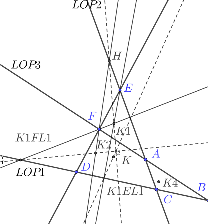
Figure 7. Construction of the most probable position, the Lemoine point of the quadrilateral determined by four lines of position (dark lines). The symmedian points of the triangles are K 1, K 2, K 3, K 4. The line through K 2 and F meets LOP 1 at K1FL1. The Lemoine point of the quadrilateral lies on the line through K1FL1 and K 2, similarly we construct the point K1EL1 and the line through K 3 etc.
From (Thas, Reference Thas2003, Theorem 1), and following the example on p166 of that paper we notice that for any i≠j the Lemoine point of the quadrilateral K satisfies
 $$(K_i K) \cap LOP_j = (K_jK_{ij}) \cap LOP_j$$
which means the line from the Lemoine point of the quadrilateral to the symmedian point of the triangle formed by omitting LOP i from the quadrilateral meets LOP j at the same point on that line as the line from one of the vertices (where the lines not i or j meet) and the symmedian point of the triangle omitting j. For any choice of a pair of i and j, i≠j this gives us a line through K. We just choose two such instances and the lines intersect at K. In Figure 7 we repeat the construction again for a different choice to demonstrate that it gives the same solution.
The Encyclopedia of Quadri-Figures gives the Least Squares Point of a quadrilateral as the point minimizing the sum of squared distances from its four basic lines as QL-P26, (van Tienhoven, Reference van Tienhoven2018). Other constructions are given as well as relations to some other known points of quadrilaterals. The Encyclopedia of Polygon Geometry lists the Lemoine point as nL-n-P6, and includes constructions (van Tienhoven, Reference van Tienhoven2019).
For the ellipses, Thas notes that the line segments KK i, i=1, …, 4 form diameters of the ellipse conjugate to the diameters through K and parallel to each LOP i respectively. From any pair of conjugate diameters (for description see Figure 17) we can construct the ellipse, for example using Rytz's construction (Ostermann and Wanner, Reference Ostermann and Wanner2012), see Figure 18.
An inspection of the proof of Theorem 1 in (Thas, Reference Thas2003) shows that it does not rely on the coefficients of the matrix being normalised, so applies to the weighted case. The case of four lines of position proceeds as before but taking the weighted symmedian point of sets of three lines as in Section 9.
11. WORKED EXAMPLE
To illustrate the process of constructing the symmedian point and an elliptical probability contour in the unweighed case we will go through a worked example. With a little practice the procedure can be done quite quickly and it tends to look much more cumbersome when written out in detail than when demonstrated. Also, there may well be further short-cuts that can be made to the procedure we give. To give an element of realism we will base our example loosely on an observation of Vega, Altair and Jupiter given as Problem 26 in (Burch and Miller, Reference Burch and Miller2014). We will assume that the variances of the errors are the same, although from the data given we could estimate the variances from the series of sights. The sights are adjusted to the same time and relative to an assumed position (AP) at one time. The LOPs and cocked hat are shown in Figure 8 as they would appear using graph paper as a plotting sheet. The horizontal axis is distance in nautical miles from the AP rather than longitude. Now zooming in on the cocked hat, Figure 9, we see this is relatively small, and also that it is obtuse and close to isosceles. We bisect the angles at A and C, we could choose any two. Next we construct the medians, Figure 10. We need the midpoints of the two sides opposite the vertices we chose in the first step, so we bisect BC and AB. These perpendicular bisectors are useful as they meet at the circumcentre O, and we need that later. Note that the perpendicular bisectors are parallel to the lines from the AP to the GPs of the bodies, so as a check we can use parallel rules to draw them.
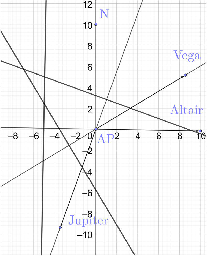
Figure 8. Worked example showing LOPs and directions to GPs of bodies. The coordinates in nautical miles are centred on the assumed position AP.

Figure 9. Now zoomed in on the cocked hat with vertices labelled A, B, C. We show the compasses construction for bisecting the angle at A. This is repeated at C and the angle bisectors meet at the incentre.
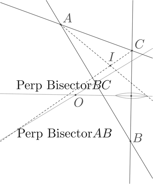
Figure 10. We bisect the line segment BC This can be done by striking an arc with radius larger than half |BC| from B and C. The line joining the intersection of the arcs is the perpendicular bisector. We do this for two sides and they intersect at the circumcentre O.
We now join the midpoint of BC to A, and the midpoint of AB to C. These are the medians. We reflect the angle bisectors in the median lines giving the symmedian lines, Figure 11. The symmedian lines intersect at the symmedian point K and we take this as our fix. Note that the triangle is close to isosceles. If it were isosceles we would find the symmedian point on the axis of symmetry, but it is not and AC, on the LOP for Jupiter, is the shorter side so K is closer to that.
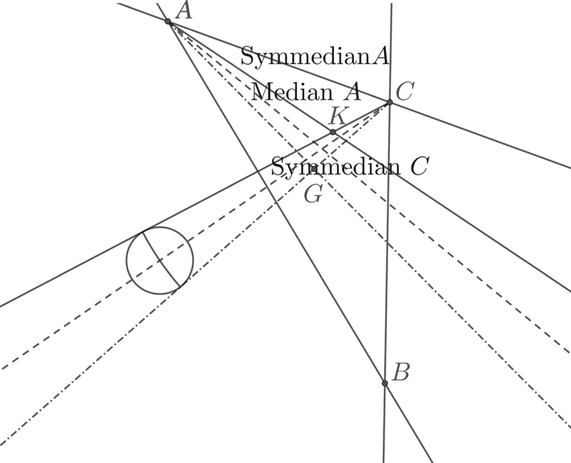
Figure 11. We join the vertices A and C to the midpoints of the opposite sides. We then reflect the angle bisectors in the median lines to form the symmedian lines. This can be done with a simple compasses procedure to copy the angle as illustrated or by measurement with a protractor. The symmedian lines intersect at the symmedian point K.
It is probably best to rub out construction lines that are not needed as otherwise the plotting sheet can get very confusing. For the next step we will need K, O, and also the centroid G, which is the intersection of the medians. Also keep the LOPs. We draw the circumcircle and the Euler line, Figure 12. We do not need to construct H, although it would be easy as we would just intersect a line through one vertex normal to the opposite LOP, with the Euler line. Instead we just strike out the distance |OG| from G on the Euler line. This point is labelled D but it is triangle centre X(381), and we just use the properties listed in ETC to construct it. We now have the orthocentric circle.
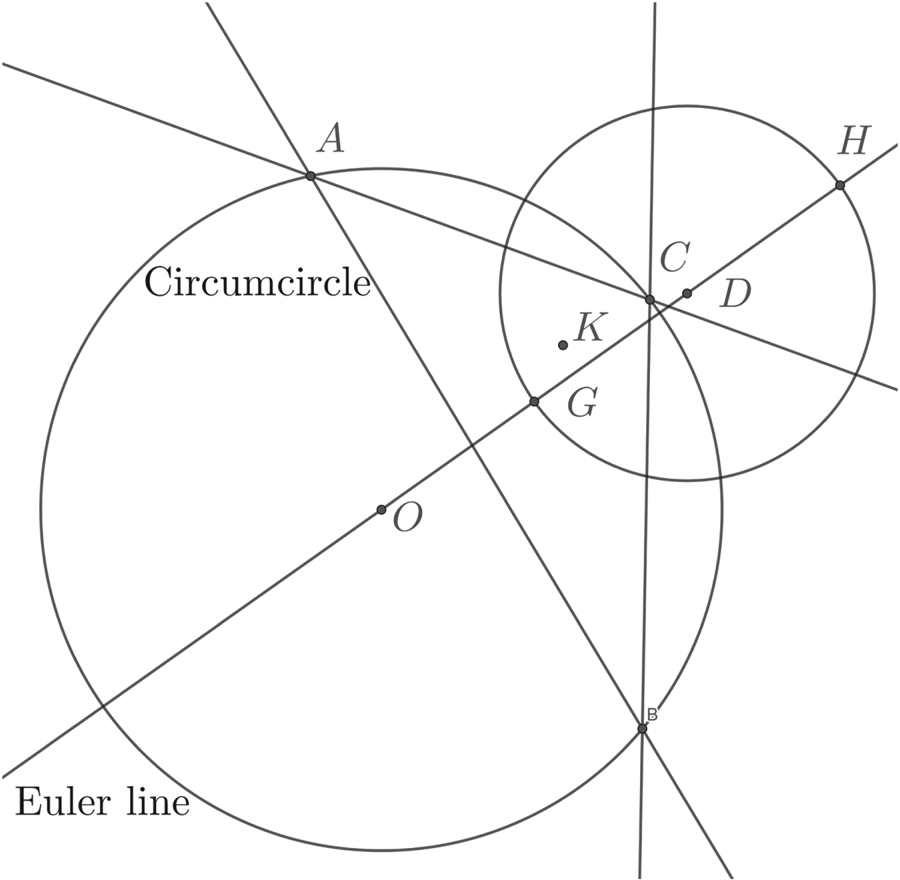
Figure 12. In preparation to find the point on the axis we draw the circumcircle through O and A (and of course B and C). The Euler line is the line through O and G. We need O the centre of the orthocentric circle. The easiest way to obtain this is to strike of the distance |OG| centred on G, labelled as D. The orthocentric circle is the circle centred on D through G.
Now we construct X(1344) just as we did in Figure 5. We draw a diameter of the circumcircle and a parallel diameter of the orthocentric circle, Figures 12 and 13. A parallel rule is an efficient way to do this and is familiar to the navigator. The line joining opposite diameters intersects the Euler line at X(1344). In our case this is quite close to K and so one should do this on a plotting sheet on a larger scale. In practice, the major axis is, as expected, nearly parallel to the longest side in this nearly isosceles obtuse triangle. In Figure 14 we construct the angle of the diagonal of the bounding rectangle of the ellipse while in Figure 15 this angle is transferred to K and the bounding rectangle and vertices of the ellipse is constructed. In Figure 16 we show how the two circle method is used to construct points on the ellipse given the vertices and centre.
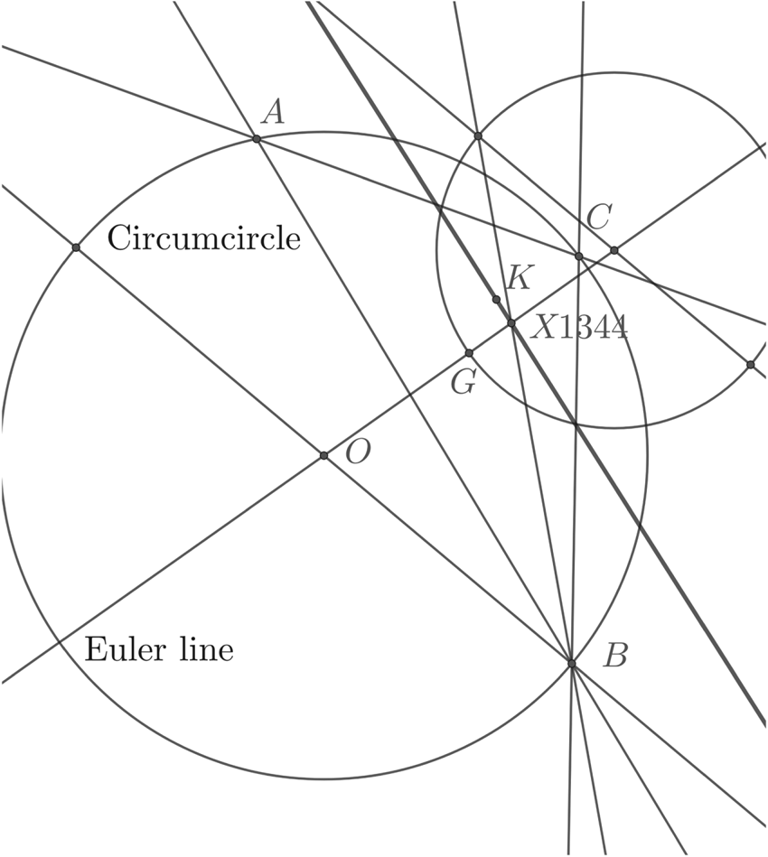
Figure 13. We now draw any diameter of the circumcircle, we chose to go through A, and a parallel diameter of the orthocentric circle. Joining opposite points where the diameters meet the circles, intersected with the Euler line, gives the incentre of similitude of the two circles, X(1344). The line joining this to K (thicker line) is the major axis.
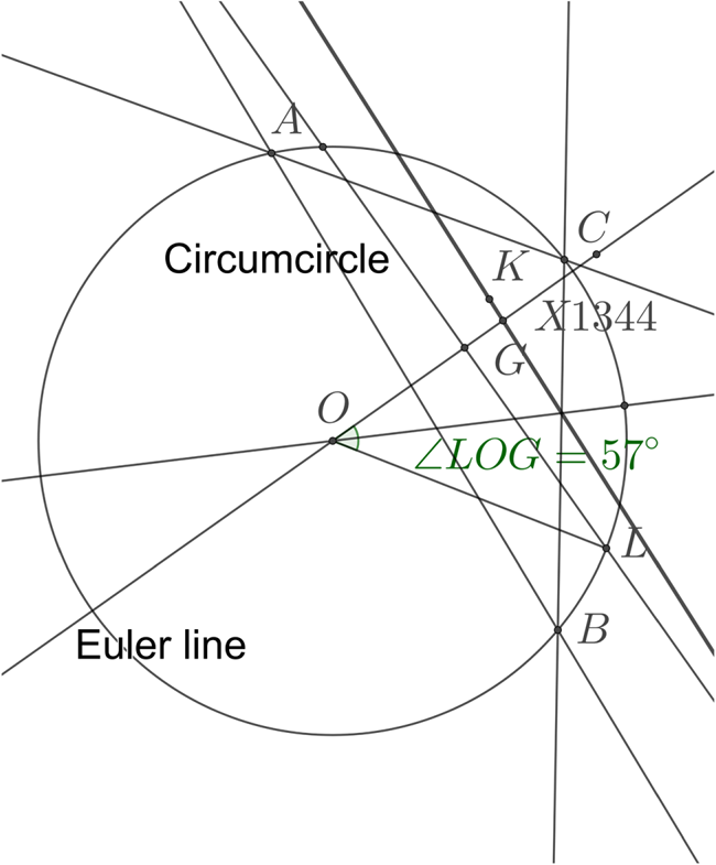
Figure 14. A perpendicular to the Euler line through G meets the circumcircle at L, and Angle LOG=57°. We bisect this angle to get ψ=28°.

Figure 15. A line is drawn through K at ψ=28° to the major axis. This is the diagonal of the enclosing rectangle (left). The rectangle is drawn with sides aligned with the axes and with the given diagonal (right).
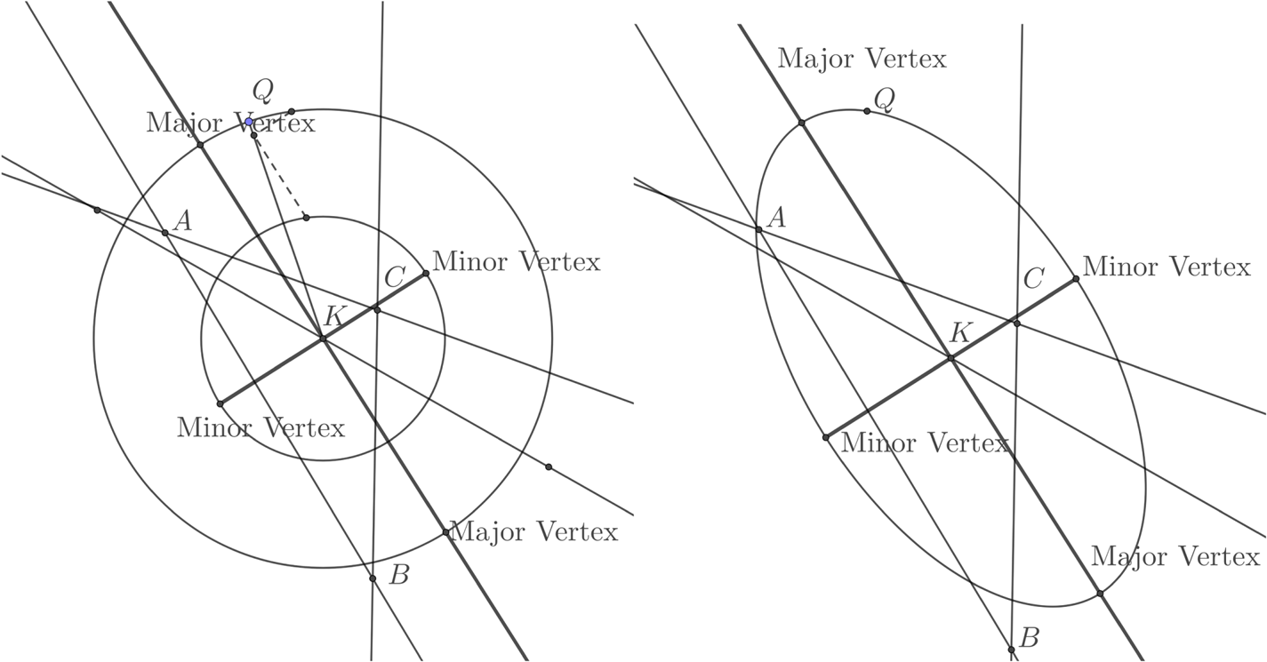
Figure 16. The ellipse is constructed using the two circle construction. For simplicity only one radial and point Q is shown (left). The final ellipse with just the LOPs (right).
While this procedure might be swiftly executed with practice we doubt it will be widely used at sea. A better approach might be to remember a set of representative cases such those illustrated in Figure 6 and this will give a reasonable estimate of the eccentricity and orientation of the ellipse. Possibly the exercise of working through the procedure of constructing the ellipse will help a navigator not just to memorise a list of examples but understand how the process works, and for some that is more likely to be retained long term than rote learning.
To improve the accuracy of navigation, we suspect that the navigator's time is better spent practising the taking accurate sights in quick succession, and recognising stars so that more LOPs can be obtained.
12. DISCUSSION AND CONCLUSIONS
We have succeeded in finding invariant descriptions for the family of ellipses, and these allow probability ellipses to be constructed using ruler and compasses construction, as can the most probable position. Importantly we gain some insight in the alignment of the major axis relative to the triangle. As we have expressed the parameters of the ellipses in terms of the angles between the lines, it is clearly not the size of the cocked hat that determines the size of the probability contour. It is the variance of the errors. While the procedure for constructing the ellipse can be performed rapidly with practice, we suggest that a navigator with time to practice is better spending that time improving the accuracy of their sights.
For the weighted case, in which the variances of the measurements differ, we see that once the weighted centroid is known, the weighted symmedian point and ellipse can be constructed by ruler and compasses. Importantly, we note that for the case of an acute triangle the weights can be chosen so that the probability contours are circular. This means that if the only three celestial bodies available are unfortunately placed so that the ellipse is highly eccentric, and the cocked hat is acute, by taking more sights of some bodies than others one can achieve circular probability contours.
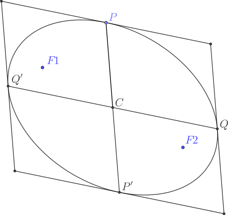
Figure 17. Conjugate diameters of an ellipse are two lines through the centre C meeting the ellipse at P and P′, and Q and Q′, so that CP is parallel to the tangent at Q and CQ parallel to the tangent at Q.
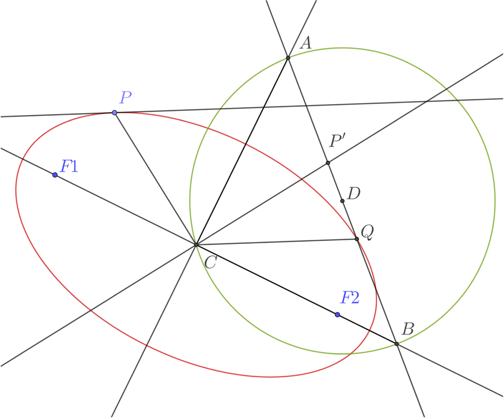
Figure 18. Rytz construction of the axes of an ellipse from conjugate diameters. Given conjugate semi-diameters CP and CQ, construct the point P′ so CP′ is orthogonal to OP and the same length. Let D be the midpoint of P′Q. The circle centred on D through C meets the line P′Q at A and B. CA and CB give the directions of the axes. The length of the semi-axes are given by |DA| and |DB|.
We have shown that using Thas's theorem one can derive a ruler and compasses construction of the most probable position and the probability ellipses for n>3 lines of position in the plane. Our cautions about the practicality of this, balanced against gaining some intuition about the direction and eccentricity of the ellipse, are valid also for this case.
For n+1 equations in n variables the solution of the least squares problem lies at the symmedian point of the simplex. For the case n=3, the tetrahedron (Sadek et al., Reference Sadek, Bani-Yaghoub and Rhee2016), for general n > 2 (Sadek, Reference Sadek2017). Applications to navigation include a position fix in three dimensional space by distances to four distant known points. More generally a construction is given for the Lemoine point for m > n + 1 equations in n variables by (Thas, Reference Thas2003).
ACKNOWLEDGEMENTS
The authors thank Herbert Prinz for providing reference (Yvon-Villarceau and Aved de Magnac, Reference Yvon-Villarceau and Aved de Magnac1877) in response to WL's query on NavList as to the earliest use of the symmedian point in the navigation literature.
FINANCIAL SUPPORT
WL would like to thank The Royal Society for the Wolfson Research Merit Award that funds research in Inverse Problems, of which this work is a spin-off.


