
Introduction
Since the late 1970s, successive satellite missions have been monitoring the Sun’s activity and recording the Total Solar Irradiance (TSI) time-series. Some of these measurements have lasted for almost three decades. In order to obtain a seamless record whose duration exceeds that of the individual instruments, the time-series have to be merged. Climate models can be better validated using such long TSI time-series which can also help provide stronger constraints on past climate reconstructions (e.g., back to the Maunder minimum). We have developed a 3-step method based on data fusion, including a stochastic noise model to take into account short and long-term correlations. Compared with previous products scaled at the nominal TSI value of ∼ 1361 Wm-2, the difference in terms of mean value over the whole time series is below 0.2 Wm-2. Similar results are obtained when comparing the various time-series in terms of solar minima. The new TSI composite, merged from several time-series, is a further development of the previous composite released by the late Dr. Claus Fröhlich. This new composite is not determined using the same algorithm, but it is statistically comparable. Indeed, we calibrate (step 3) our new TSI composite using the previous PMOD/WRC TSI composite.
Results and Discussion
Our TSI composite is produced using a new statistical approach, which is based on three key steps. Here, the steps are summarised, but a comprehensive discussion of the algorithm is given by Montillet et al. (2021a; 2021b; 2021c; 2021d). The first step relies on the data fusion of multiple observations based on a Bayesian framework and Gaussian processes. Our composite spanning the last four decades is obtained in the second step by linking the sub-time-series resulting from the first step. The last step is the application of wavelet filtering to correct some unwanted correlations in the fused observations (i.e. bandwidth noise). The robustness of our approach is guaranteed via a careful modelling of the TSI observations during the data fusion process.
During the construction of the composite, we followed the base assumptions developed for the previous PMOD/WRC composite which are:
- Correction of the early HF measurements from NIMBUS 7 to account for its early increase, degradation and non-exposure dependent increase (Fröhlich and Lean, 1998; Fröhlich, 2006).
- Assessment of the early increase and degradation of ACRIM-I (Fröhlich, 2006).
- Tracking of ACRIM-II to ACRIM-I by comparison with only HF, corrected as described in the first bullet (earlier versions also used ERBS and the model, see Fröhlich (2000) and Fröhlich (2003)).
- Detailed assessment of the influence of the many operational interruptions in the ACRIM-II record (Fröhlich, 2004).
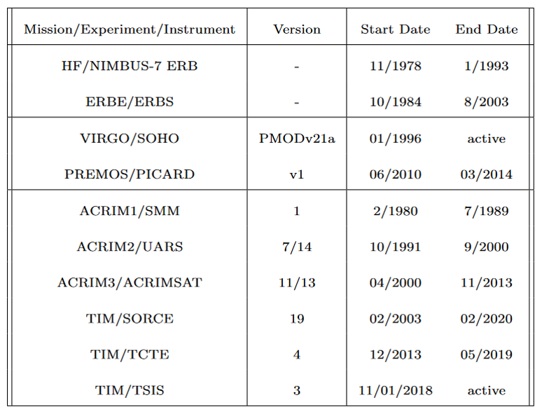
The details of these corrections can be found in Fröhlich, 2006 and also widely discussed in ISSI WS2005. With these corrections on HF, ERBS, ACRIM-I and ACRIM-II, we then merged all the available data using the new algorithm as shown in Figure 1 and Table 1.
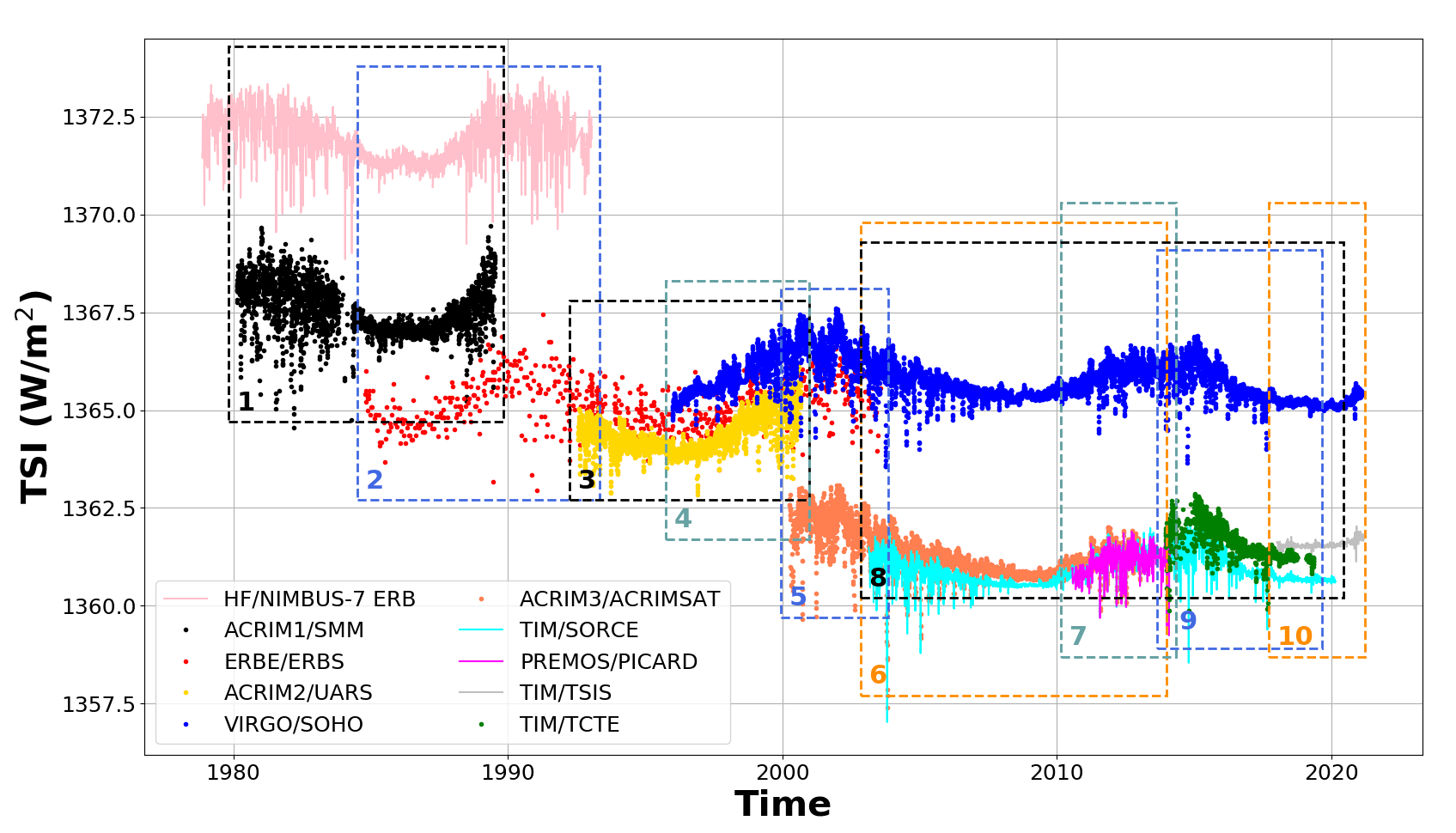
Figure 1. Overview of all data recorded by various missions in the last four decades and used in the PMOD/WRC TSI composite.
Table 1. Information about the datasets used in the PMOD/WRC TSI composite.
We performed a statistical comparison with previous released products, namely by Dudok de Wit et al. (2017), Dewitte and Nevens (2016) and Fröhlich (2006) known as Composite 1 (C1), Composite 2 (C2) and Composite 3 (C3) in the following. The PMOD/WRC TSI composite is referred to as the Composite PMOD-Data Fusion or CPMDF1, and after applying the wavelet filter in step 3, it is referred to as CPMDF2. Figure 2 displays the composite time-series overlaying the previous PMOD/WRC TSI composite (C3). Estimates of TSI at the solar minimum across the various solar cycles from 1980 to the present are shown in Table 2.
Table 2. Estimate of TSI at the solar minimum during the last 41 years from the TSI time-series (mean μ and standard deviation σ) released by Dudok de Wit et al. (2017) (C1), by Dewitte and Nevens (2016) (C2) and by Frohlich (2006) (C3). The new TSI composite is referred to as CPMDF1, and after using the wavelet filter, to CPMDF2. The difference in irradiance between solar minima (SM) from consecutive solar cycles (e.g., ∆I22/23−21/22) is also displayed with the uncertainties (bold text).
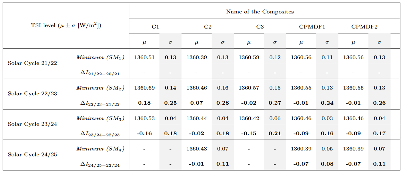
Note that the solar minima are underlined in Figure 2 (see yellow boxes). The solar minimum periods are chosen according to Dudok de Wit et al. (2017) and Finsterle et al. (2021) by looking at the lowest value in the yearly-averaged sunspot number and then averaging the irradiance values over a one-year interval centered on that date. When comparing the mean difference between the product and our time-series over the various solar minima, the new composites agree with C1 by 0.09±0.04 Wm-2, C2 by 0.08±0.06 Wm-2, and C3 by 0.03±0.01 Wm-2. The same order of magnitude is obtained if the wavelet filter (see CPMDF2) is used. The difference is marginal for C1, C2 and C3, within the 1-sigma interval of 0.2 Wm-2. This value is defined in Finsterle et al. (2021), and is based on the various versions of the PMO6v products released by PMOD/WRC over the last decades. Note that C2 is re-scaled to the nominal TSI value of 1361 Wm-2 adopted by the IAU in 2015 (Resolution B3; Prsã et al., 2016), averaged over Solar cycle 23. By applying this process, the calculated offset is equal to 2.44 Wm-2 which is due to the calibration based on the absolute level estimated from DIARAD/SOVIM. C1 and C3 are closest to the nominal TSI value (below 0.1 Wm-2) averaged over Solar cycle 23 due to their intrinsic processing. The results have slightly improved by ∼ 0.02 Wm-2 when applying the wavelet filter.
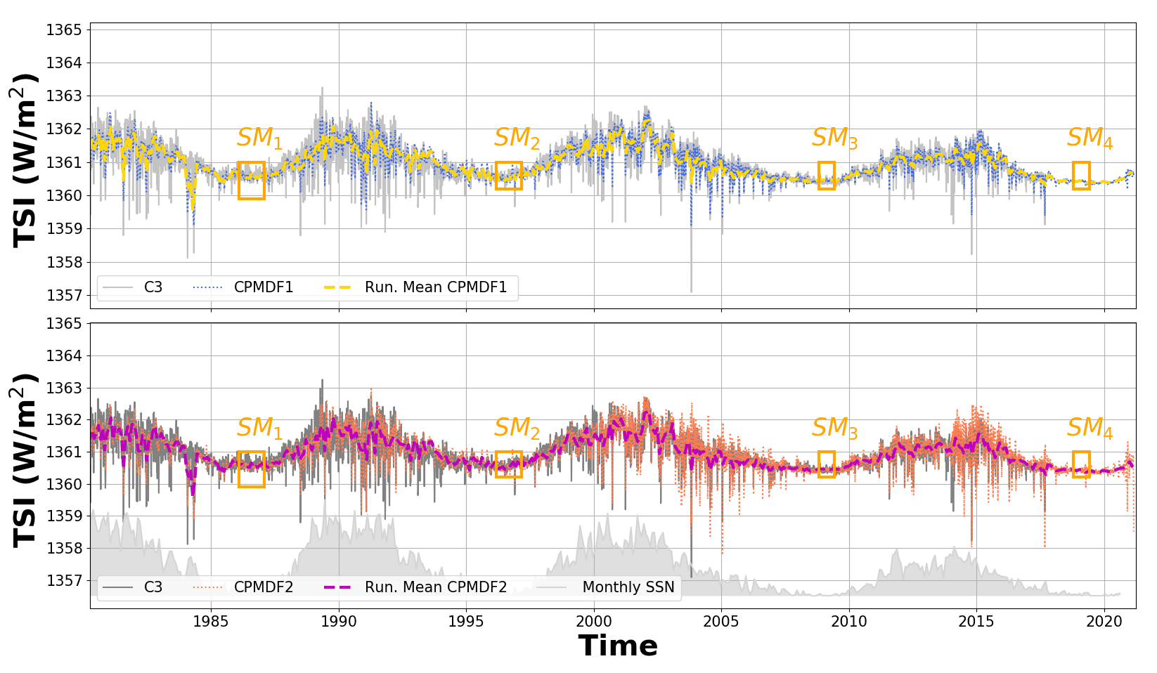
Figure 2. The new Composite (CPMDF1, blue) without and with a wavelet filter CPMDF2 (orange) based on merging 41 years of TSI measurements. For comparison, C3 (Fröhlich, 2006) is also shown (grey line). A 30-day running mean of CPMDF1 is shown as a yellow/purple dashed line. The orange boxes are associated with the solar minima (SM) for each solar cycle described in Table 2. For context, the monthly sunspot numbes are also displayed.
Then, we perform a power spectrum density (PSD) analysis in Figure 3 of the composite time-series. We can analyse four frequencies (11.5 years, 27, 9 and 7 days ) related to solar activity, which are described by Fröhlich et al. (1997). The frequency associated with 11.5 years is the Schwabe cycle. The quasi 27-day solar cycle is caused by the sun’s differential rotation, presumably first observed by Galileo Galilei or Christoph Scheiner in the first half of the 17th century. The spectrum is divided into three areas (i.e. boxes A, B and C) following the previous assumptions on the stochastic properties of the TSI observations (and the solar cycle). The definition of the three areas also follows the description of the photospheric activity. The latter, associated with granulation, super-granulation and meso-granulation (Fröhlich et al., 1997), generates fluctuations in TSI at different time-scales. Due to our 1-day resolution, frequencies associated with phenomena lasting a few hours or less (i.e. granulation) cannot be observed.
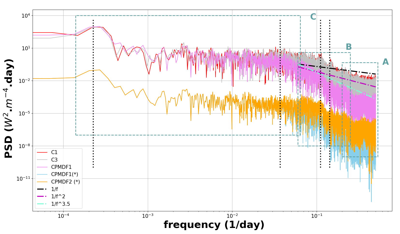
Figure 3. Power Spectrum Density (PSD) of TSI C1 (Dudok de Wit et al., 2017), C3 (Frohlich, 2006), together with the new TSI composite produced with the current method, CPMDF1, and application of the wavelet filter, CPMDF2. The asterisk (∗) depicts time-series that are shifted by re-scaling the amplitude by −4 W2m−4 day in the log-log plot. Boxes A, B and C refer to the different sections of the PSD: A is centered on the high frequencies (∼3 days) showing the flattening of the PSD; B is the power-law which is mainly due to coloured noise (correlations between 20 and 6 days) within the time-series; C emphasises the low frequencies associated with the stochastic and deterministic parts of the solar cycle and long-term correlations. The dashed lines are the various power-law models when varying the exponent only for indication. The vertical doted lines (black) mark the frequencies at 11.5 years, 27, 9 and 7 days (l to r).
Box A shows a flattening of the curve at high frequencies. The time-series is displayed with a daily and minute sampling rate. For comparison, we also show the PSD of C3 and CPMDF2. The PSD of the products with a daily sampling rate experience the same flattening at high frequencies, whereas the monotonic behaviour of the curve disappears in the sub-daily frequency band. Shapiro et al. (2017) argued that the high frequencies are associated with the radiometer technical characteristics and satellite movements (i.e. open/close shutter, orbit revolutions). Fröhlich et al. (1997) also show that the solar noise flattens in this frequency band. We can then conclude that the flattening is due to the low-sampling rate in the TSI composites.
Box B is the power-law or the frequency ramp (between 0.06 and 0.25 day−1). This phenomenon is due to the existence of correlations in the observations. It is arguable that this power-law describes the long-term correlations (i.e. over years), due to the ramp spanning frequencies over only a few days (4 – 20 days). Therefore we can only speculate which underlying process can generate it. For example, it could be an unknown diffusion process associated with the sun’s activity which could be modelled with a specific coloured noise called Matérn process. Nonetheless, the steepness of this ramp shows the degree of correlation or the type of stochastic noise within the time-series, by fitting a power-law model such as S(f ) ∼ 1/f^β . The exponent β defines the type of coloured noise: flicker noise corresponds to β equal to 1, a random walk to β equal to 2, and white noise with β equal to 0 (Montillet et al., 2021b; 2021c; 2021d). Figure 3 displays that the steepness of the ramp is above 2, and even above 3 for the new TSI composite (CPMDF1). The factors due to the increased steepness are discussed by Montillet et al. (2021c; 2021d). In summary, the data fusion process behaves as a wideband filter. The resulting noise properties depend on the transition band of the filter so that the white noise is transformed into a power-law noise with a variable exponent β. In addition, one can show that the power-law is also included in the PSD of C1, C2 and C3 with a much less steeper ramp. Montillet et al. (2021c; 2021d) shows the relationship with the long-term dependencies over years associated with the photospheric activity. This relation is also discussed by Dudok de Wit et al. (2017).
Box C is associated with the low frequencies (0.06 – 0.00015 day−1). They are assumed to be mostly related to the deterministic part of the solar cycle and the long-term correlations (i.e. lasting up to years). In addition, this frequency band also contains some of the coloured noise linked to long-term correlations (over years) due to the sun’s activity.
In conclusion, we have merged 41 years of satellite observations using data fusion in order to produce a TSI composite time-series, which can be used to study the solar cycle modulation and the Earth’s energy budget. We performed a time-frequency comparison of our new TSI composite with previous releases. The results show that the mean difference over the solar minima is below the 1-sigma confidence interval of 0.2 Wm-2, i.e. a maximum of 0.09 Wm-2 with C1 and a minimum of 0.03±0.01 Wm-2 with C3.
Data Availability and Additional Information
The VIRGO/SOHO webpage, illustrating our new method to retrieve TSI, was updated in Feb. 2022. The previous TSI composite webpage was archived in May 2022 but can still be accessed (TSI composite archived webpage).
Our TSI composite is produced using a new statistical approach, which is based on three key steps. The new composites, CPMDF1 and CPMDF2, are accessible on the below ftp server. Note that within the file, the term “TSI after corr.”, means that we have applied a wavelet filter to the TSI composite as described in Step 3 of the algorithm. The term, “TSI after corr.”, refers to CPMDF2. Note: As some browsers no longer allow ftp links to be opened, please use an ftp programme to access the data instead.
ftp://ftp.pmodwrc.ch/pub/data/irradiance/virgo/TSI/TSIcomposite/
The TSI composite, C3, can be retrieved from the PMOD/WRC archive and is available on request from Dr. W. Finsterle. The TSI composite, C1, can be downloaded from the ISSI Bern solar irradiance website, while C2 is available on request from Dr. S. Dewitte.
The data related to the monthly/daily mean sunspot numbers can be retrieved from the Royal Observatory of Belgium website. Time-series from the TIM /SORCE, TCTE/TIM and TIM/TSIS, and ACRIM (www.acrim.com; sunclimate.gsfc.nasa.gov/instrument/acrim) experiments are available from their respective websites.
PMODv21a (also called PMODv8) is available at: ftp://ftp.pmodwrc.ch/pub/data/irradiance/virgo/TSI/.
PREMOS (v1) data can be accessed from the PICARD archive.
References
Dewitte, S., Nevens, S., (2016), The Total Solar Irradiance Climate Data Record, Astrophys. J., 830 (1), 25. http://doi.org/10.3847/0004-637x/830/1/25
Dudok de Wit, T., Kopp, G., Frohlich, C., Scholl, M., (2017), Methodology to create a new total solar irradiance record: Making a composite out of multiple data records, Geophys. Res. Lett., 44, 1196–1203, https://doi.org/10.1002/2016GL071866
Finsterle, W., Montillet, J., Schmutz, W., Sikonja, R., Kolar, L., & Treven, L. (2021), The total solar irradiance during the recent solar minimum period measured by SOHO/VIRGO. Scientific Reports, 11 (7835), https://doi.org/10.1038/s41598-021-87108
Frohlich, C., Scholl, M., (2017), Methodology to create a new total solar irradiance record: Making a composite out of multiple data records, Geophys. Res. Lett., 44, 1196–1203, https://doi.org/10.1002/2016GL071866
Fröhlich, C., and J. Lean, (1998), The Sun’s total irradiance: Cycles and trends in the past two decades and associated climate change uncertainties, Geophys. Res. Lett., 25, 4377-4380.
Fröhlich, C., (2000), Observations of irradiance variability, Space Science Reviews, 94, 15-24.
Fröhlich, C., (2003), Long-term behaviour of space radiometers, Metrologia, 40, 60-65.
Fröhlich, C., (2004), Solar Irradiance Variability, in Solar Variability and its Effect on climate, Chapter 2: Solar Energy Flux Variations, AGU, Geophysical Monograph,Series No. 141, 97-110.
Fröhlich, C. and J. Lean, (2004), Solar Radiative Output and its Variability: Evidence and Mechanisms, Astron. and Astrophys. Rev., 12, pp. 273-320, https://dx.doi.org/10.1007/s00159-004-0024-1
Fröhlich, C., (2006), Solar Irradiance Variability Since 1978: Revision of the {PMOD} Composite During Solar Cycle 21, Space Sci. Rev., 125, 53-65, https://dx.doi.org/10.1007/s11214-006-9046-5
Fröhlich, C., (2012), Total solar irradiance observations, Surveys in Geophysics, 33, 453-473, https://dx.doi.org/ 10.1007/s10712-011-9168-5
Mekaoui, S., Dewitte, S., (2008), Total solar irradiance measurement and modelling during cycle 23. Sol. Phys., 247, 203–216, https://doi.org/10.1007/s11207-007-9070-y
Montillet, J.-P., Finsterle, W., Schmutz, W., Haberreiter, M., Sikonja, R., (2021a), Data fusion of Total Solar Irradiance composite time series using 40 years of satellite measurements: First results, EGU General Assembly 2021, online, 19–30 Apr 2021, EGU, https://doi.org/10.5194/egusphere-egu21-4382
Montillet, J.-P., Finsterle, W., Kermarrec, G., Sikonja, R., Haberreiter, M., Schmutz, W., Dudok de Wit, T., (2021b), https://doi.org/10.1002/essoar.10509108.1
Montillet, J.-P., et al., (2021c), https://www.essoar.org/doi/10.1002/essoar.10508721.2
Montillet, J.-P., Finsterle, W., Kermarrec, G., Sikonja, R., Haberreiter, M., Schmutz, W., Dudok de Wit, T., (2021d), Data dusion of Total Solar Irradiance composite time series using 41 years of satellite measurements, https://agupubs.onlinelibrary.wiley.com/doi/abs/10.1029/2021JD036146
Montillet, J., Finsterle, W., Schmutz, W., Haberreiter, M., Dudok de Wit, T., Kermarrec, G., Šikonja, R., (2022), Composite PMOD Data Fusion – updated September 2022, Version 1.0. Interdisciplinary Earth Data Alliance (IEDA), https://doi.org/10.26022/IEDA/112687, accessed 2022-10-14.
Prsã, A., Harmanec, P., Torres, G., Mamajek, E., Asplund, M., Capitaine, N., … Stewart, S.G., (2016), Nominal values for selected solar and planetary quantities: IAU 2015 Resolution B3, Astronomical Journal, 152 (2), 41, https://doi.org/10.3847/0004-6256/152/2/41
Shapiro, A., Solanki, S., Krivova, N., Cameron, R., Yeo, K., Schmutz, W., (2017), The nature of solar brightness variations, Nat. Astron., 1 , 612–616, https://doi.org/10.1038/s41550-017-0217-y